
Composite Integration#
It usually doesn’t pay to go to higher-order polynomials (e.g., fitting a cubic to 4 points in the domain). Instead, we can do composite integration by dividing our domain \([a, b]\) into slabs, and then using the above approximations.
Here’s an illustration of dividing the domain into 6 slabs:
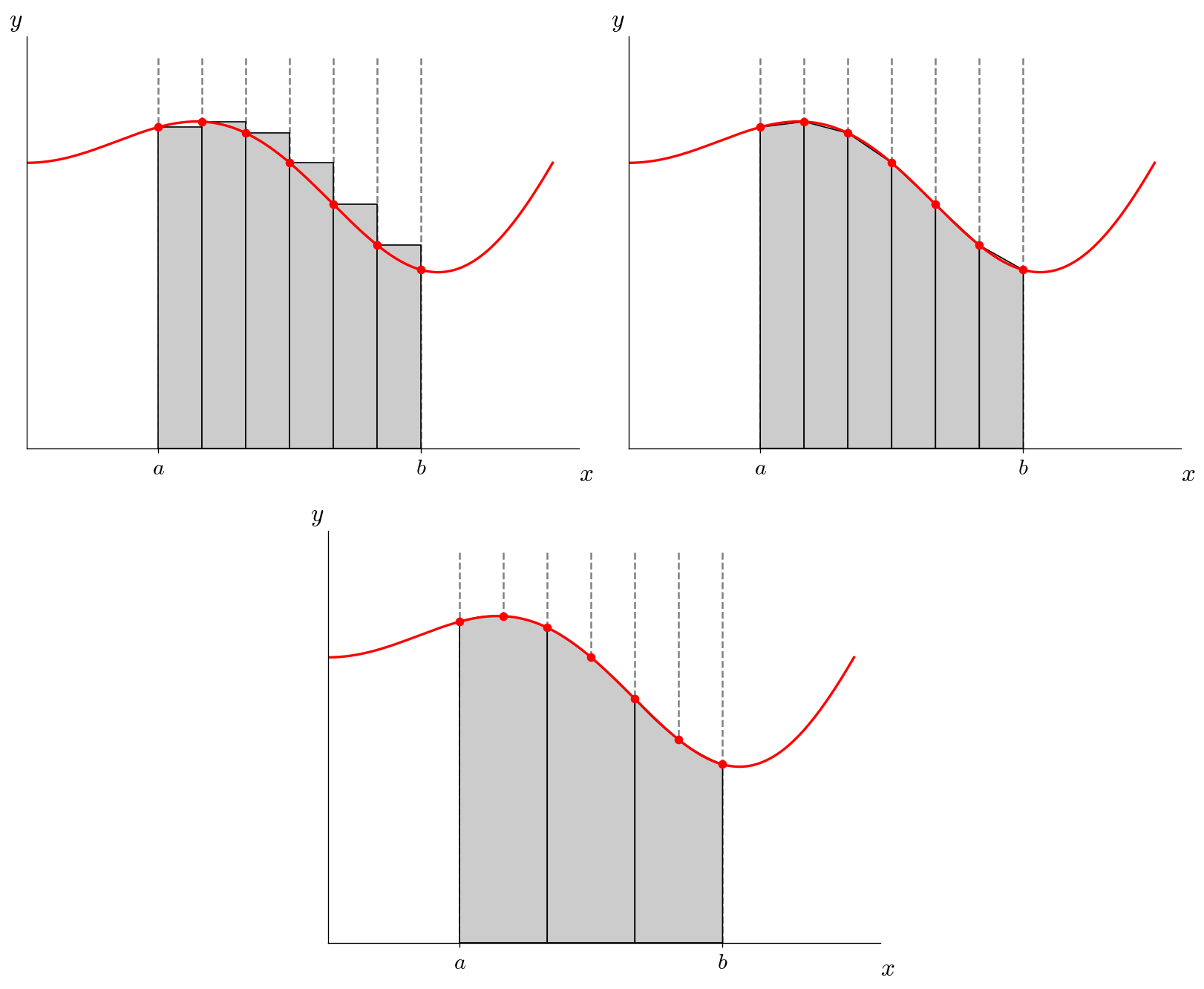
Imagine using \(N\) slabs. For the rectangle and trapezoid rules, we would apply them N times (once per slab) and sum up the integrals in each slab. For the Simpson’s rule, we would apply Simpson’s rule over 2 slabs at a time and sum up the integrals over the \(N/2\) pair of slabs (this assumes that \(N\) is even).
The composite rule for trapezoid integration is:
and for Simpson’s rule, it is:
Example:
For the function in the previous exercise, perform a composite integral using the trapezoid and Simpson’s rule for \(N = 2, 4, 8, 16, 32\). Compute the error with respect to the analytic solution and make a plot of the error vs. \(N\) for both methods. Do the errors follow the scaling shown in the expressions above?
First let’s write the function we will integrate
def f(x):
    return 1 + 0.25 * x * np.sin(np.pi * x)
Now our composite trapezoid and Simpson’s rules
def I_t(x):
    """composite trapezoid rule.  Here x is the vector
    of coordinate values we will evaluate the function
    at."""

    # the number of bins is one less than the number
    # of points
    N = len(x)-1

    I = 0.0

    # loop over bins
    for n in range(N):
        I += 0.5*(x[n+1] - x[n]) * (f(x[n]) + f(x[n+1]))
    return I

def I_s(x):
    """composite Simpsons rule.  Here x is the vector
    of coordinate values we will evaluate the function
    at."""

    # the number of bins is one less than the number of
    # points
    N = len(x)-1

    # we require an even number of bins
    assert N % 2 == 0

    I = 0.0

    # loop over bins
    for n in range(0, N-1, 2):
        dx = x[n+1] - x[n]
        I += dx/3.0 * (f(x[n])+ 4 * f(x[n+1]) + f(x[n+2]))
    return I
Integration limits
a = 0.5
b = 1.5
The analytic solution
I_a = 1 - 1/(2 * np.pi**2)
Now let’s run for a bunch of different number of bins and store the errors
# number of bins
N = [2, 4, 8, 16, 32, 64, 128, 256]

# keep track of the errors for each N
err_trap = []
err_simps = []

for nbins in N:

    # x values (including rightmost point)
    x = np.linspace(a, b, nbins+1)

    err_trap.append(np.abs(I_t(x) - I_a))
    err_simps.append(np.abs(I_s(x) - I_a))
Now we’ll plot the errors along with the expected scaling
err_trap = np.asarray(err_trap)
err_simps = np.asarray(err_simps)
N = np.asarray(N)

fig = plt.figure()
ax = fig.add_subplot(111)

ax.scatter(N, err_trap, label="trapezoid rule")
ax.scatter(N, err_simps, label="Simpson's rule")

# compute the ideal scaling
# err = err_0 (N_0 / N) ** order
fourth_order = err_simps[0] * (N[0]/N)**4
second_order = err_trap[0] * (N[0]/N)**2

ax.plot(N, second_order, label="2nd order")
ax.plot(N, fourth_order, label="4th order")

ax.set_xscale("log")
ax.set_yscale("log")

ax.legend()
ax.set_xlabel("number of bins")
ax.set_ylabel("error")
Text(0, 0.5, 'error')
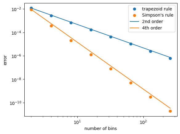
One thing to note: as you make the number of bins larger and larger, eventually you’ll hit a limit to how accurate you can get the integral (somewhere around N ~ 4096 bins for Simpson’s). Beyond that, roundoff error dominates.
C++ implementation#
A C++ implementation of Simpson’s rule for this problem can be found at: zingale/computational_astrophysics